Table of Contents
API for the JEA Engine
Key Features
- On-the-fly controllability including process, algorithm configuration, evaluation metrics, and search space.
- Supports full parametrics, random and quasi-random sampling/sensitivity analyses, single-/multi-objective optimisation.
- Standard and truncated probabilistic distributions include: integer: Bernoulli, Binomial, Geometric, Hypergeometric, Pascal(a.k.a. Negative binomial), Poisson, and Discrete uniform, and continuous: Beta, Cauchy, Chi-squared, Exponential, F, Gamma, Levy, Log-normal, Normal, Pareto, T, Triangular, Continuous uniform, and Weibull
- Sampling methods include: Shuffling, LHS, Sobol, Halton, Random Walk (one parameter at a time, single step, N x (d + 1)), Morris (one parameter at a time, random step size, N x (d + 1)), and Saltelli (Sobol N x (d + 2))
- Performs sensitivity assessment using: Morris method, Sobol method, and ordinary multivariate linear regression. Regression parameters and standardized coefficients (a sensitivity measure) are calculated for every output variables, applied automatically on each complete optimisation, parametric or sampling runs, or calculated on report request of partial runs.
- Reported data include regression results, descriptive statistics, and frequency histogram.
- Full project data including the exploration history and the details of the explored solutions in JSON format.
- Access control and project/data sharing (for JEA Web only).
- Accessible online using REST API or integrated into users programs as a standalone library (license required).
Concept
Algorithm as a Service
The JEA engine with the JEA Web interface is what we call “Algorithm as a Service”. It is equivalent to the traditional program libraries in which the algorithms can be accessed through function calls. The JEA engine is exactly the same, albeit it can be called from any programming or scripting languages, as long as they support HTTP transactions. This provides ultimate flexibility for using the algorithms, with the additional benefits of project sharing and multi-dimensional data analyses features.
The Algorithm as a Service approach also separates the algorithm engine from the evaluation models. The algorithm engine does not know how each candidate solutions are evaluated. It is down to the user and the client program to conjure up numbers and send them to the engine, so that it can tell which solutions are superior and to which direction it should explore further. This design gives unlimited opportunities to novel approaches such as hybrid methods, robust optimisation, surrogate modelling, and multi-disciplinary decision making.
The typical process of using the engine contains the following steps:
- Gain access to the service by checking in (with existing key) or logging on (with user credentials).
- Prepare the project definition, which includes details of the design variables, evaluation results as reported by the client program, and “fitness” metrics such as objective and constraint functions, the algorithm settings, and auxiliary information about the project.
- Create the project on the Engine using the “Create” command
- Start the project using the “Start” command
- Inquire and retrieve any pending evaluation cases from the Engine
- Run simulations on the evaluation cases, and collected outputs as defined in the project.
- Submit evaluation results to the Engine
- Repeat 5, 6 and 7 until one of the termination criteria is met, or satisfactory results have been found.
- Project data can be retrieved from the Engine, or viewed online with JEA's multidimensional data visualization tools.
Engine states diagram
Once created, a JEA project can go through a number of states, controlled by the user with relevant commands, or by the progression of the exploration process. The diagram below is an illustration of the states of the project. Clicking on the commands will take you to the related parts of the documentation.
<html> <img src=“http://www.jeplus.org/wiki/lib/exe/fetch.php?w=450&tok=c5a93f&media=docs:jea_engine_states_diagrams.png” alt=“JEA state flow diagram” usemap=“#Map” style=“display:block; margin: 0 auto” /> <map name=“Map” id=“Map”>
  <area alt="Create" title="Create command" href="http://www.jeplus.org/wiki/doku.php?id=docs:jea:create_project" shape="rect" coords="185,45,249,65" />
  <area alt="Start" title="Start command" href="http://www.jeplus.org/wiki/doku.php?id=docs:jea:start_project" shape="rect" coords="194,130,252,152" />
  <area alt="Start" title="Start command" href="http://www.jeplus.org/wiki/doku.php?id=docs:jea:start_project" shape="rect" coords="63,237,120,258" />
  <area alt="Start" title="Start command" href="http://www.jeplus.org/wiki/doku.php?id=docs:jea:start_project" shape="rect" coords="105,281,161,302" />
  <area alt="Reset" title="Reset command" href="http://www.jeplus.org/wiki/doku.php?id=docs:jea:reset_project" shape="rect" coords="1,207,48,233" />
  <area alt="Reset" title="Reset command" href="http://www.jeplus.org/wiki/doku.php?id=docs:jea:reset_project" shape="rect" coords="310,152,371,175" />
  <area alt="Reset" title="Reset command" href="http://www.jeplus.org/wiki/doku.php?id=docs:jea:reset_project" shape="rect" coords="403,208,450,233" />
  <area alt="Pause" title="Pause command" href="http://www.jeplus.org/wiki/doku.php?id=docs:jea:pause_project" shape="rect" coords="256,212,308,233" />
  <area alt="Resume" title="Resume command" href="http://www.jeplus.org/wiki/doku.php?id=docs:jea:resume_project" shape="rect" coords="252,280,314,302" />
  <area alt="Stop" title="Stop command" href="http://www.jeplus.org/wiki/doku.php?id=docs:jea:terminate_project" shape="rect" coords="157,304,198,326" />
  <area alt="Stop" title="Stop command" href="http://www.jeplus.org/wiki/doku.php?id=docs:jea:terminate_project" shape="rect" coords="285,314,333,338" />
  <area alt="Cancel" title="Cancel command" href="http://www.jeplus.org/wiki/doku.php?id=docs:jea:cancel_project" shape="rect" coords="202,305,260,328" />
  <area alt="Cancel" title="Cancel command" href="http://www.jeplus.org/wiki/doku.php?id=docs:jea:cancel_project" shape="rect" coords="336,302,396,322" />
  <area alt="Delete" title="Delete command" href="http://www.jeplus.org/wiki/doku.php?id=docs:jea:delete_project" shape="rect" coords="161,425,226,444" />
  <area alt="Delete" title="Delete command" href="http://www.jeplus.org/wiki/doku.php?id=docs:jea:delete_project" shape="rect" coords="233,425,298,445" />
</map> </html>
REST API
The REST API calls are summarized in the table below. For details of each transaction, click on the command names and the data description links. Please note that [the sub-pages require update]
Note:
- Base Access Point URL A:
https://api.ensims.com/jea_web/api - Base Access Point URL B:
https://api.ensims.com/users/api
| Group | Command | OP | BaseAP | Path | Auth | Data | Return |
|---|---|---|---|---|---|---|---|
| General | Version info inquiry | GET | A | /info | none | none | Version info |
| Auth (Users API) | Check in with existing key | POST | B | /checkin | JWT in cookie | none | Auth return |
| Log on with credentials | POST | B | /logon | none | User credential | Auth return | |
| Managing Projects | List existing projects | GET | A | /projects/{own/all} | JWT in cookie | none | List of project IDs |
| Upload File | POST | A | /upload | JWT in cookie | Multipart form data | File Info | |
| Download File | GET | A | /download/<file ID> | JWT in cookie | none | file contents | |
| Project Command | Create command | POST | A | /command | JWT in cookie | Command object | Response |
| Update project | POST | A | /command | JWT in cookie | Command object | Response | |
| Start project | GET | A | /start/<project ID> | JWT in cookie | none | Response | |
| Pause project | GET | A | /pause/<project ID> | JWT in cookie | none | Response | |
| Resume project | GET | A | /resume/<project ID> | JWT in cookie | none | Response | |
| Terminate project | GET | A | /terminate/<project ID> | JWT in cookie | none | Response | |
| Cancel project | GET | A | /cancel/<project ID> | JWT in cookie | none | Response | |
| Reset project | GET | A | /reset/<project ID> | JWT in cookie | none | Response | |
| Delete project | GET | A | /api/delete/<project ID> | JWT in cookie | none | Response | |
| Project Data | Get status | GET | A | /status/<project ID> | JWT in cookie | none | Project Status |
| Get project definition | GET | A | /definition/<project ID> | JWT in cookie | none | Command Object | |
| Get report | GET | A | /report/<project ID> | JWT in cookie | none | Project Report | |
| Get Data | GET | A | /data/<project ID> | JWT in cookie | none | Data archive | |
| Get partial Data | GET | A | /data/<project ID>/<version>_<generation> | JWT in cookie | none | Data archive (partial) | |
| Run Evaluation | Get awaiting jobs | GET | A | /jobs/<project ID> | JWT in cookie | none | Simulation jobs |
| Submit simulation results | POST | A | /eval | JWT in cookie | Simulation Results | Engine Response |
Access the API
The REST API is accessible with any HTTP client that allows you to assign data to the header and the body of each request. JEA uses only the GET and the POST methods. In general, when a data object is sent in the request's body, the POST method is used. To experiment and test the API commands, we recommend Postman. A Postman collection of transactions showing all the commands is available to download here.
Depending on the programming language you are using, there are numerous HTTP client to choose from. In this document, the examples of using curl and Requests for Python are provided in the descriptions of each transaction. Here is a quick example using the get version info command.
Browser
Since this command does not require authentication, you can try it in a web browser by typing in the following URL:
https://api.ensims.com/jea_web/api/info
If the service is accessible, you will receive a page containing the following text:
{
  "Title" : "JEA Web API",
  "Description" : "an optimisation service provided by ENSIMS Ltd.",
  "Major" : 1,
  "Minor" : 0,
  "Revision" : 2,
  "Release" : "stable",
  "Update" : 0,
  "Notice" : "(C) 2016-2019, Energy Simulation Solutions Ltd. All rights reserved."
}
curl
Send the same command using curl:
curl https://api.ensims.com/jea_web/api/info
The same text will be return with successful execution.
Requests
Make sure Requests is correctly installed in your Python environment, and run the following the lines:
>>> import requests
>>> r = requests.get('https://api.ensims.com/jea_web/api/info')
>>> r.json
The Technicals
NSGA2 tuning
NSGA2 (Deb et al. 2002) is one the best known and widely used algorithms for multi-objective optimisation. The key trick is the Nondominated Sorting method (hence the name), which is proven to be highly effective in ranking competing objectives. One deficiency of the original NSGA2 is that it does not provide a way for handling constraints efficiently. This is addressed in JEA using the Stochastic Ranking method.
Non-dominated Sorting and Stochastic Ranking
Constraint handling is a topic that attracts lots of attention from algorithm designers. The efficiency of constraint handling is measured by not only how quickly feasible solutions are found, but also the quality of those feasible solutions. If a strategy pushes too hard for meeting the constraints, it may hamper exploration for better objective values. On the other hand, if it is too lenient, too much time may be wasted on infeasible solutions. The balance depends on the nature of the problem, so a perfect strategy may not exist. However, from our research we found one of the best strategies in terms of robustness of adaptability to different problems, is Stochastic Ranking (Runarsson and Yao, 2000).
Stochastic Ranking is a probabilistic strategy to rank solutions with the different objective and constraint values. Its original form is designed for one objective against one constraint. In order to make it work with NSGA-II, the following steps are taken:
- All constraints are scaled (normalized) and then aggregated so that the infeasibility (constraint violations) is measured as a value in [0, 1].
- Infeasibility is used as an additional objective and sorted with Non-dominated Sorting with all other objectives. This produces an initial ranking order of all solutions.
- Stochastic Ranking is then applied to the initial rank of each solution (treated as its objective value) and its aggregated infeasibility value. This produces the final ranking of the solutions.
The benefit of this slightly complex arrangement is that it works well with problems with any number of objectives (including single objective) and constraints, and unconstrained problems. The user can use a single parameter, what we call “Objective Bias”, to control the level of the push for feasibility.
Two configuration parameters directly affect the behaviour of NSGA2 with Stochastic Ranking. objectiveBias controls the ranking bias between Pareto ranking and infeasibility scores. A value of zero means solutions with lower infeasibility score is better, disregard of the Pareto ranking result. elitismTollerance controls if infeasible solutions can be selected as elites (see next section) or not. If a positive value is assigned, e.g. 0.1, it means solutions with infeasibility scores up to 0.1 may be selected as elites.
Pareto Archived elitism
Evolutionary algorithms are stochastic in nature. The user has little control over which direction or what solutions to explore next. Quite often promising solutions may appear in one generation and then disappear for good in the subsequent iterations. Elitism is a method for preserving good solutions. Basically, it selects cases from a pool of known solutions and inserts them back into the working population.
In Pareto Archived elitism, all known solutions on the global Pareto front are stored. They form the pool from which the elitism operator picks “elites”. In JEA, the maximum number of elites and whether they can include infeasible solutions can be controlled with parameters.
Two configuration parameters directly affect the behaviour of elitism. globalElitism controls from which pool the elite solutions are selected. If set to true (default), selection will be made in the global archive; otherwise it is limited to the current population. elitismTollerance also affect how elitism works. It has been explained in the previous section.
Uncertainty and Sensitivity Analyses
JEA supports Uncertainty Analysis through implementing various sampling methods and a broad range of probabilistic distributions. Statistics can be performed on the simulation results of the random sample to give uncertainty estimations. The statistical methods implemented in JEA is limited to descriptive statistics and multiple linear regression at present. The statistics are calculated automatically at the end of each optimisation, parametric or sampling run. A subsequent Report request will retrieve the statistical data as part of the engine report.
Three Sensitivity Analysis methods have been implemented in JEA. These are regression analysis, the Morris method, and Saltelli's variance based method (a.k.a. Sobol method). The latter two are triggered when their corresponding sampling methods are used. The former is applied to any complete or partial runs. Sensitivity results are included in the project report.
Sampling methods
JEA supports five sampling methods: pseudo-random sample through shuffling, simple symmetric random walk (one variable, one step at a time with equal probability), Latin hypercube sampling (LHS), Sobol sequence, and Halton sequence, plus a variable step random walk as required by Morris Method, and Saltelli sampling for the Sobol Method.
Lots of information can be found online relating to these methods. Notes and references of the methods are as below:
- pseudo-random sample: a sample is created by shuffling the full list of permutations and select the first N cases. This method is only available to problems whose search space size is no greater than 100,000.
- Random walk: (see Wikipedia entry) a simple symmetric random walk method is implemented. The sample size (N) determines the number of starting points, which is generated by Latin hypercube sampling. The number of steps equals to the number of parameters (D) plus 1. So, the total sample size is N x (D + 1).
- Latin hypercube sampling (LHS): (see Wikipedia entry) LHS is a highly efficient sampling method. As a rule of thumb, a sample size of 10 times the number of parameters will give a reliable estimate of the population mean.
- Two quasi-random low dependency sequences are available: Sobol (see Wikipedia entry) and Halton (see Wikipedia entry).
- Sampling method specific to Morris Method is a symmetrical random walk with variable step sizes.
- The Saltelli sampling for Sobol sensitivity analysis. Details see Wikipedia entry
Probabilistic distributions
The JEA engine supports a wide range of continuous and integer probabilistic distributions. These are very useful for uncertainty and sensitivity analyses.
Syntax
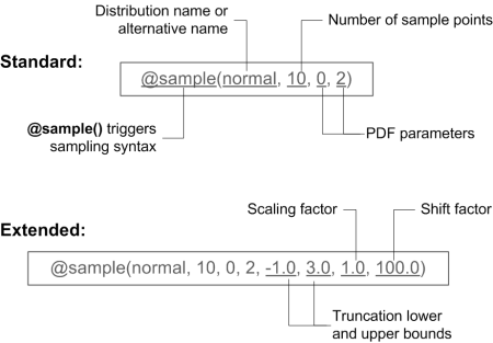
The probabilistic distribution functions to be used in the “valueStr” field of parameter definition require the following general syntax:
@sample(<distribution name>, <N sample points>, <PDF parameter1>, ...)
Or in the extended form with four additional fields defining the truncation, scaling and shifting of the distribution:
@sample(<distribution name>, <N sample points>, <PDF parameter1>, ..., <truncation lower bound>, <truncation upper bound>, <scaling factor>, <shifting factor>)
The example below shows its use:
Equal probability sample
One of the key features of the JEA engine is that it works exclusively on discrete parameter values, even if the parameter is continuous in nature. Normally, when you define the parameter values using the list (e.g. {1, 3, 4, 5}) or the range (e.g. [1:1:5]) syntax, user-specified discrete values are stored with the parameter. When a parameter is defined as a continuous probabilistic distribution function, however, you must instruct JEA how many sample points it should consider, so that a sample of discrete values can be drawn from the distribution.
JEA uses a deterministic approach to sample a distribution. First, the value range of the parameter is divided into N equal probability sections. Then, the median values of each section are taken as the sample points. For example, the diagram below shows how the values in the sample set of 10 points of a normal distribution are drawn.
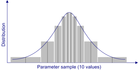
In fact, for a sample set of 10 points, the 5th, 15th, 25th, …, and 95th percentiles are drawn as the values. This method means that for a given sample definition, the set of points are invariable, i.e. the repeated runs will contain the same set of values. Also, note that many continuous distributions have long tails, which may lead to the sample set containing values that are not considered practical. (See the extremities in the diagram above for an example.) To avoid those values, you need to apply truncation to such distributions.
Continuous distributions
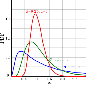
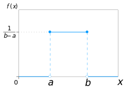
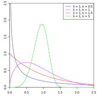
This table summarizes the available continuous distributions available in JEA: (all charts are from the respective Wikipedia pages)
Integer distributions
This table summarizes the available discrete distributions available in JEA: (all charts are from the respective Wikipedia pages)
| Distribution | Names | Param1 | Param2 | Param3 | Example | Reference (Wikipedia) |
|---|---|---|---|---|---|---|
| Bernoulli (Binomial n=1) distribution | bernoulli, 1, dbe | p | - | - | @sample(bernoulli, 10, 0.5) | Reference |
| Binomial distribution | binomial, 3, dbi | trials | p | - | @sample(binomial, 10, 20, 0.5) | 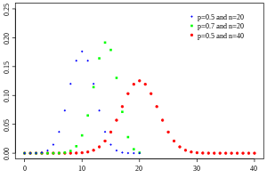 |
| Geometric distribution | geometric, 9, dge | p | - | - | @sample(geometric, 10, 0.3) | 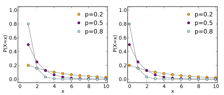 |
| Hypergeometric distribution | hypergeometric, 10, hypergeo, dhy | Population size | number of successes | sample size | @sample(hypergeometric, 10, 100, 30, 10) | 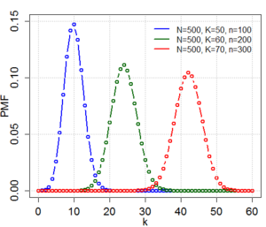 |
| Negative Binomial (Pascal) distribution | pascal, 13, negativebinomial, dpa | number of successes ® | probability of success (p) | - | @sample(pascal, 10, 20, 0.5) | 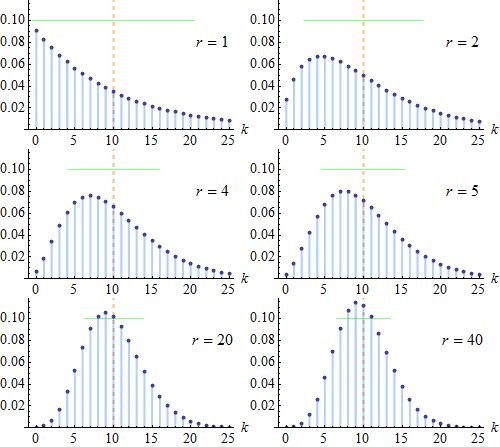 |
| Poisson distribution | poisson, 16, dpo | Poisson mean | - | - | @sample(poisson, 10, 5) | 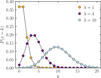 |
| Discrete uniform distribution | duniform, 20, discreteuniform, dun | lower limit | upper limit | - | @sample(duniform, 10, 2, 8) | 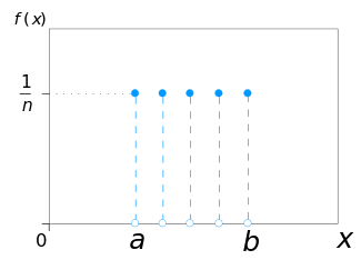 |
Discrete distribution by values
When parameter values are specified not using the “@sample()” syntax, their distribution is considered as uniform, i.e. each value has the equal probability to take place. Sampling is done by applying Discrete uniform distribution on the indexes of the values.
Truncation, Scaling and Shifting
The latest implementation of the sampling function support Truncation, scaling and shifting of the PDF functions. These transformations can be applied to all PDF functions except the discrete distribution defined by listing values (see above).
To enable these transformations, add four extra parameters to the probabilistic functions defined above, in the sequence of Umin, Umax, Scale, and Shift. Truncation, scaling and shifting are applied in this order, too. Care should be taken to assign the correct parameter values. For example, to truncate, scale and then shift a normal distribution, define it as:
@sample(normal, 10, 0, 2, -1.0, 3.0, 1.0, 100.0)
Where for the normal distribution mean = 0.0 and sd = 2.0, truncate it to the range of [-1.0, 3.0], do not use scaling (scale = 1.0), but shift the range to +100.0.
Truncation is applied to continuous and integer distributions in the same manner. To disable it, provide the values of Umin and Umax so that Umin >= Umax. For example, @sample(normal, 10, 0, 2, 0, 0, 1, 0) is equivalent to @sample(normal, 10, 0, 2), where no truncation, nor scaling or shifting takes place.
If scaling and/or shifting are applied to integer distributions, the output sample values will be decimal numbers instead of integers. This allows specifying decimal values that follow integer distributions.
